Background
In reliability engineering, “too little, too late” is not an option, especially in some industrial process facilities where asset failures can have significant consequences –financial and otherwise. Reliability engineers are now turning to data analysis and Monte Carlo simulation to predict and prevent failures.
San Antonio, Texas-based Zachry Industrial is an engineering and construction firm serving the refining, chemical, power, and pulp and paper industries. The Maintenance and Reliability Services Department at Zachry supports clients in the reliability, availability, and maintenance of their plant assets.
Over the years, Zachry reliability engineers working in client process plants have observed that failure rates can abruptly increase due to unintended and unrecognized changes in repair quality, or operating or process conditions. The changed failure rates were slow to be recognized, often only after several additional failures had occurred. Zachry engineers then undertook to recognize failure rate trends at the very earliest time, so that negative failure trends could be immediately turned around. All new failures trigger an automatic analysis so that results with statistical significance are known prior to repair. This permits the data analysis to influence inspection and repair plans. This immediate and selective intervention of reliability degradation allows elimination of failures that otherwise would occur.
Developing new methods with @RISK
Conventional failure time analysis methods are slow to detect abrupt shifts in failure rates and require larger datasets than what are often available, so new methods were developed. One method uses Poisson distribution in reverse to identify failure times that do not fit the distribution. Probability values (p-values) quantify the likelihood that failure times are unusual relative to random variation. Failure times with good statistical strength of evidence are “alarmed” as issues of interest.
“As new data arrives, analysis is done contemporaneously, not because there is a problem of interest, but to see if there may be a problem of interest,” said Kevin Bordelon, Senior Director of Operations at Zachry Industrial.
Data for trend detection is drawn from asset work order data for individual assets residing in a client’s Enterprise Resource Planning systems. These assets can range from large machines to small instruments, so there can be tens of thousands of individual assets within a manufacturing plant. While the total database is huge, each individual asset dataset can be extremely small. Traditional methods either can’t be used on very small datasets, or confidence intervals are so wide as to make them unreliable. (Confidence intervals show how wrong a value may be).
Every maintenance action request for a particular asset triggers extraction of historical data for that asset. Using prior maintenance action dates, Poisson p-values are automatically generated. The idealized “textbook” expectation for repairable equipment is such that the Poisson distribution characterizes failure counts over time intervals. This textbook expectation is exactly the opposite of what is needed to identify the unusual special cause failures of interest, so the Poisson is used in reverse as a null hypothesis distribution. Low Poisson p-values suggest failure times are unlikely to be random variation from the textbook expectation; therefore, they are likely to be special cause failures that should be investigated.
“Using datasets much smaller than normal and using unfamiliar data analysis methods make having a statistically sound measure of confidence in the results absolutely essential. This is done by forming probability distributions around the p-values. These distributions show the variation in the p-value if the equipment’s reliability condition could be resampled thousands of times. Of course this is physically impossible, but is easily done by computer simulation through @RISK.” explains Bordelon. “Combining Excel’s flexibility with @RISK allows a single @RISK simulation to simultaneously generate probability distributions around all of the numerous p-values.”
Kevin Bordelon
Zachry Industrial
Probability values and maps
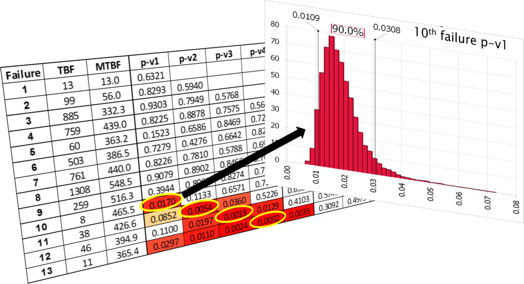
Failure times (dates) are used to determine the time between failures (TBF). Each failure has a TBF value that defines that failure. Upon each failure, that TBF produces a p-v1 value. This is the probability of one or more failures occurring in the TBF interval when the mean time between failure (MTBF) is determined from all prior TBF values. A look back of two TBF values determines a p-v2 value. This is the probability of two or more failures occurring with an interval of time equal to the sum of the last two TBF values. Upon each failure, this process is repeated for all prior TBF values, producing a probability map as seen in the figure (below).
The probability map is progressively developed with each failure. Upon each failure, the p-values are calculated using only the then existing data, being blind to future data. This allows developing trends to be seen as failures are experienced. Missed opportunity to take action also stands out as significant probability values can be traced backward in time. For example in the figure below, the last four failures had continually smaller and smaller p-values, indicating increasing strength of statistical evidence of reliability degradation. With only the data that existed upon the 10th failure, the p-v1 suggests the one quick failure is unlikely to be random variation and is likely to be a special cause failure that should be investigated. Had this been done, the next three failures could have been avoided.
“To say that a single fast-acting failure establishes a statistically significant trend is unprecedented and demands confidence limits around the measurement. But @RISK solves the confidence problem by efficiently developing probability distributions for every p-value in a single simulation,” Kevin Bordelon says. “The methods for obtaining confidence levels around the probability values are inconceivable without @RISK, and to accept the new analysis methods you have to have confidence in the results.”