
When performing a cost risk analysis study, one of the key results is the amount of extra monetary resources that is to be added to the project cost baseline to guarantee that the budget is not exceeded at a certain confidence level. Good project risk management strategies must take this into account.
After defining the uncertain variables and risk events that affect the cost performance of the project, we can run a Monte Carlo simulation with @RISK to find out what the range of the total project cost is. Simulation results can help us to explain the risk exposure that we have in the total cost of the project. The most popular statistics are the mean (average cost), the most likely cost, and the 10th and 90th percentiles.
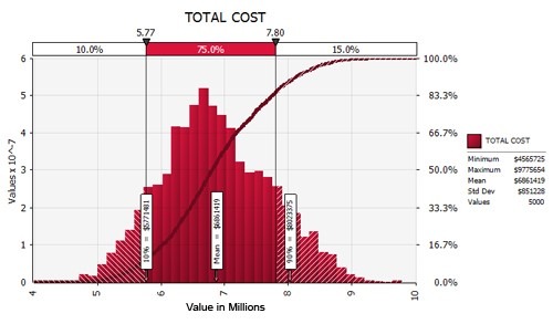
To determine the contingency to be allocated to the project, we need to define what confidence level we would like to achieve: The higher the contingency level, the larger amount of contingency needed. For example, in the figure above, we are reporting the total cost of the project. Here we can observe that we are showing the 85th percentile that corresponds to a total cost of $7.8M (right delimiter). We can say that there is only a 15% chance that we will exceed $7.8M, or alternatively, we have an 85% chance that the total cost will be less than or equal to $7.8M. In the same figure we can also see that the 90th percentile of the total project cost is $8.02M. We can say then that in order to increase our confidence level from 85% to 90%, we will need to add $220,000 to the total cost.
The calculation of the contingency is then accomplished by using the base cost estimate (BE) before the risk analysis was implemented, and the expected cost (EC) of the simulated results.
Some practitioners separate the contingency into two components: engineering allowance, and management contingency.
Engineering allowance (EA) is the difference between the expected cost and the base estimate:
EA = EC – BE
Management contingency (MC) is calculated using the difference between the cost at certain confidence lever (Cp) and the base estimate:
MC = Cp – EC
In our example, our BE = $6.5M; therefore, engineering allowance EA = EC – BE = 6.86M – 6.5M = $0.36M.
For the calculation of management contingency, we use a confidence level of 85% so Cp(85%) = $7.8M; therefore, MC = Cp – EC = 7.80M – 6.86M = $0.94M.
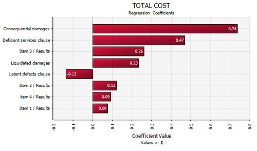
In many situations, the suggested contingency might be excessive, so the need for a mitigation study is necessary. We can use the sensitivity analysis tool in @RISK to detect the key drivers affecting our total cost. This is valuable information so that we can concentrate our efforts in reducing the impact of risk events and uncertainties to the total cost. Below, we see a tornado graph with the most important drivers. The analyst will then explore the appropriate mitigation strategies and assess their implementation cost. A second simulation can be run to assess the effectiveness of the proposed mitigation plan, and compare the pre-mitigated and post-mitigated cost distributions.
Explore @RISK for yourself by download our free 15-day free trial.