
In Part II of this series, we mentioned the existence of an analytic method to calculate the Efficient Frontier of a portfolio. Here we provide the formulas for this method.
As for other methods to calculate the Efficient Frontier, this method requires knowledge of the variance-covariance matrix of the set of assets, as well as the expected return and standard deviation (volatility) of the asset returns. The variance-covariance matrix is of course itself generally calculated from the standard deviations of the returns of individual assets and the correlation matrix between those returns.
Denoting the vector of expected returns by e, the variance-covariance matrix by V, and its inverse by VINV, and letting U denote the unit vector (consisting of ones, with the same dimension as the number of assets), then the vectors of weights (g and h, below) have returns of 0% and 100% respectively and the optimal portfolio is the vector g+rh, for any given desired level of return, r.
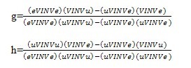
(For simplicity of presentation in the above formula, where the transposes of vectors are required for the matrix multiplication, these have not been shown.)
Since analytic formulas allow the easy implementation of sensitivity analysis, we show in the chart below the position of the optimal curve when it is assumed that equity returns are lower than historic figures case and with higher volatilities (the raw data is not shown here, but the portfolio is assumed to consist of bills, bonds, and equities).
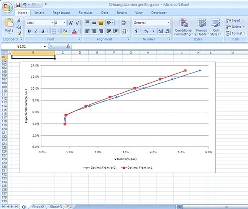
The advantages of such analytic methods include their computational efficiency, and the ease with which sensitivity analysis can be conducted (for example, that associated with parameter uncertainty). The main disadvantage is the inability to include constraints in the analysis.