
In Part I, combining simulation and decision tree analysis techniques was introduced. But what does that actually give you? What meaningful results are created to justify the work? Obviously there are good things to come, or I wouldn’t be bringing it up!
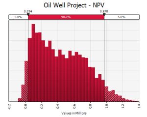
A regular spreadsheet model can produce a distribution of outcomes like this:
But as we know there may be fundamental decisions in a project that can’t be easily included in the static structure of a spreadsheet model. A decision tree analysis can generate an optimal policy like this:

But this only shows a single estimate of the expected return for that particular decision path.
Now we look at our hypothetical decision tree (an oil project, say) and decide there should actually be an uncertain value for one node. Perhaps a lognormal distribution for the amount of oil produced by a well in its first year. A RiskLognormal() function is placed into the spreadsheet to replace the constant return value. Make the return in the root node an @RISK Output, then go ahead and run a simulation!
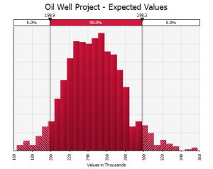
The optimal policy is still in affect, but now the actual value of the project will change based on the sampled value of this distribution during the simulation. This can be analyzed in two ways – either by creating a distribution of the expected value of the optimal policy, or a distribution of the actual values the optimal policy generates. The distinction is due to the treatment of chance nodes. In a deterministic model, a chance node returns the expected value of that node based on the likelihood of following each path and each path’s expected value. When the distributions are sampled during a simulation the expected value of the effected chance nodes changes. These expected values are then carried through the tree, resulting in a distribution of the expected return based on the optimal policy.
Alternatively @RISK can step through the individual chance node branches (with or without probability distributions in the model – the chance nodes have essentially already included discrete distributions to the model) to ultimately generate specific values that can be generated by the optimal path. In this case the decision tree is followed along a particular path until reaching the end node. The value at the specific end node is recorded by @RISK.
The distribution of the expected value of the recommended decisions might look something like this:
While the distribution of actual values, arguably more useful from a risk analysis point of view, might look like this:
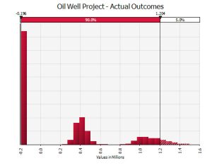
Notice how this graph gives very useful information to a decision-maker regarding their exposure to different/adverse outcomes. By combining the brute power of Monte Carlo simulation with the flexibility of decision tree structures a rich picture of possible outcomes ensues. In this instance the three (simplistic) outcomes of an empty well, reasonable returns and excellent returns are represent in the three clusters.
Try it out for yourself by downloading your 15-day free trial of the DecisionTools Suite.
Article: Getting the Full Picture Combining Monte Carlo Simulation with Decision Tree Analysis - Part 1
