
This article offers a simple and concise explanation of the Monte Carlo simulation, a technique that combines statistical concepts (random sampling) with the ability of computers to generate pseudo-random numbers and automate calculations, for basic cost engineering.
The key to Monte Carlo simulation is to create a mathematical model of the system, process, or activity to be analyzed – identifying those variables (model inputs) whose random behavior determines the overall behavior of the system. Once these inputs or random variables have been identified, an experiment is carried out which consists of generating random samples (specific values) for these inputs and analyzing the behavior of the system in response to the values generated. After repeating this experiment ‘n’ number of times, we will have ‘n’ number of observations on the behavior of the system, which will be useful to understand how the system works.
Let us look at an example of a Monte Carlo simulation cost model with continuous random variables where the model will assume we are calculating the contingency reserves for a temporary COVID-19 hospital construction project. These temporary projects have the same cost structure, but the values change from region to region. Because of variability, engineers must do a contingency analysis for each project. Typically, a percentage of the total will be used as a contingency, and we will try to improve this approach.
To infer the distributions of each cost element, historical data is ideal. However, in this type of application, there is typically not enough data for an automated fit. Therefore we will use expert judgment or the results of analyzing suppliers' bids to construct the input distributions.
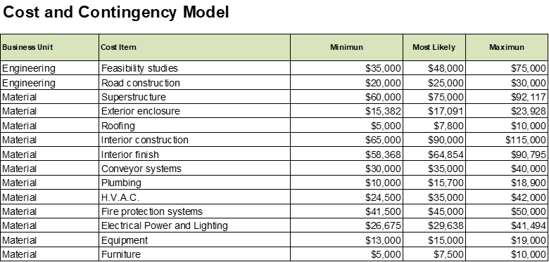
The following image shows a partial list of the cost elements in the example, each with a minimum, most probable, and maximum value. This data can be used to set up three-point distributions which are the most popular in cost engineering.
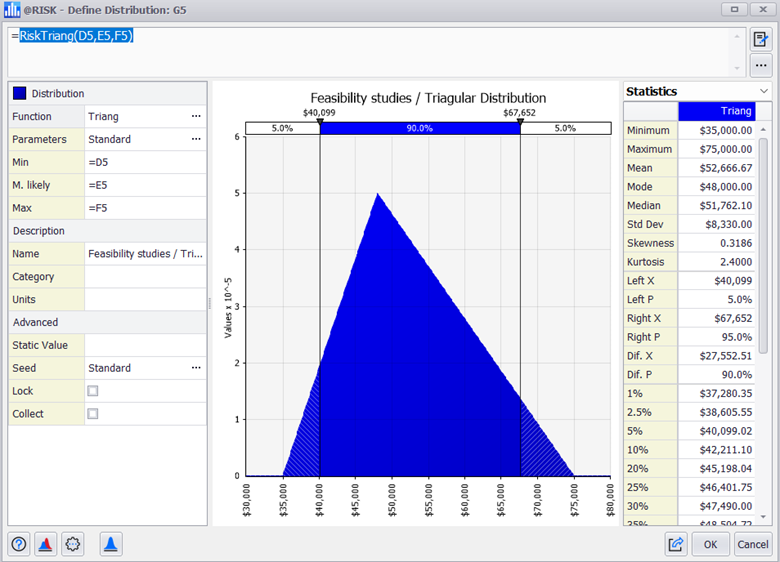
The next step is to add a column to set up a probability distribution for each cost element. After selecting the Triangular distribution and setting its three parameters: minimum, most likely, and maximum, we would get a correctly designed distribution. To improve the fit of the distribution, we can change alternative parameters such as the static value in the Excel cell (otherwise it will use the mean) or specialized parameters.
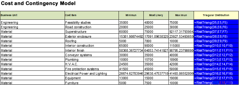
We can copy and paste the distribution formula into the cells of all the cost elements with uncertainty and verify that the formula parameters are set correctly.
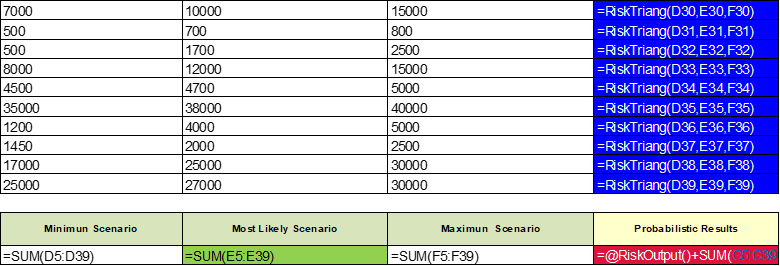
A total budget will be generated by adding up all distributions and declaring it as the Monte Carlo simulation model's output. This requires selecting the output menu and setting the name.
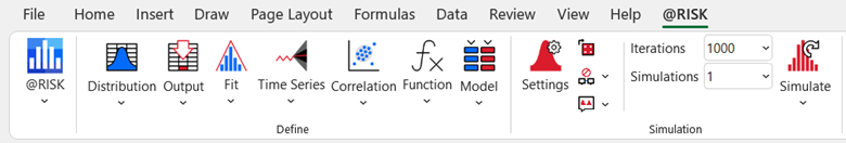
Now that we are ready to run the simulation, let's use 1000 iterations in this first test.
Once the process is finished, @RISK makes the results available with graphs, such as a histogram, and we can compare the original most probable budget against our expected value from the probabilistic model.
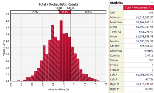
It is recommended to use the concepts of Expected Value (mean of the simulation results) and the percentile with the risk level established by the company's PMO policies, in this case the 80% percentile. The difference between the P80 and the Expected Value would give us the value of the PMO contingency reserve.

Conclusion for Basic Cost Engineering
Evidently, we can see a more interesting and justifiable technique for the calculation of contingencies; although we need to also consider that in this model, we have not considered the effect of unplanned risk events and we have reduced the model to a single distribution (Triangular).
Future articles will explain how it is possible to extend the cost engineering model by comparing it with other similar distributions or by adding a risk register that considers low probability and high impact events.
Explore @RISK by downloading a 15-day free trial.
