
Effective Grantsmanship for Research Funding
Hear from Dr. Yulia Levites on key considerations for your research grant During a recent webinar with Dr. Yulia Levites, Assistant Professor Health Services, Research,...
Resources
Check out the latest news and resources for our data solutions including NVivo, @RISK, DecisionTools Suite, XLSTAT, Citavi, Sonia, Tevera, and more.
Hear from Dr. Yulia Levites on key considerations for your research grant During a recent webinar with Dr. Yulia Levites, Assistant Professor Health Services, Research,...

Qualitative data analysis is an essential aspect of many research projects. However, the term "qualitative data" can mean different things to different people, depending on...

Revolutionizing Business Innovation with NVivo When gathering qualitative data, it’s often hard to determine the emotional undertones of the messages. In the financial industry in...
Developing a literature review is one of the most important — and difficult — components of the research process. A well-executed literature review helps you...

Creating an elevated, personalized experience for their students Higher education institutions are continuously busy coordinating field placement for students studying health, education, and other practice-based majors. This detailed process...

The All-in-One Writing and Reference Tool One of the most difficult aspects of research-based writing is keeping all your references organized. Whether you’re a PhD...

Identifying possibilities and actioning on strategic scenarios in manufacturing Welcome to a fascinating expedition into Monte Carlo simulation use in manufacturing, a powerful method for...

Basing product decisions on how consumers feel about a good or service sounds like a no-brainer, but the reality of conducting sentiment analysis and uncovering...

Discover the @RISK advantage In the dynamic field of financial services where things can change in an instant, it’s critical that financial analysts stay on...
Which qualitative content analysis methods should you choose to make sense of your data? What best practices should you adopt for each method? In the...

Three popular use cases for generative AI Generative artificial intelligence (AI) is impacting every conceivable type of application, content, and industry, and according to a...

Learn how using the Monte Carlo method in @RISK can improve your decision analysis and solve industry challenges in consumer goods, manufacturing, finance, insurance, and...
Many experts in qualitative research begin their careers in academia, science, or public policy. Katrina Noelle, founder and president of the qualitative market research consulting...
From sentiment analysis to statistical significance, this example case study shows the power of NVivo with XLSTAT. Survey data often contains a wealth of valuable...
Elevate your research experience with Citavi – because your writing deserves nothing less As a researcher, you’re no stranger to citations; but it can be...

Update Your XLSTAT Version to Unlock Smarter, Better, and Faster Insights Make more informed product decisions and improve your overall market research experience with the...
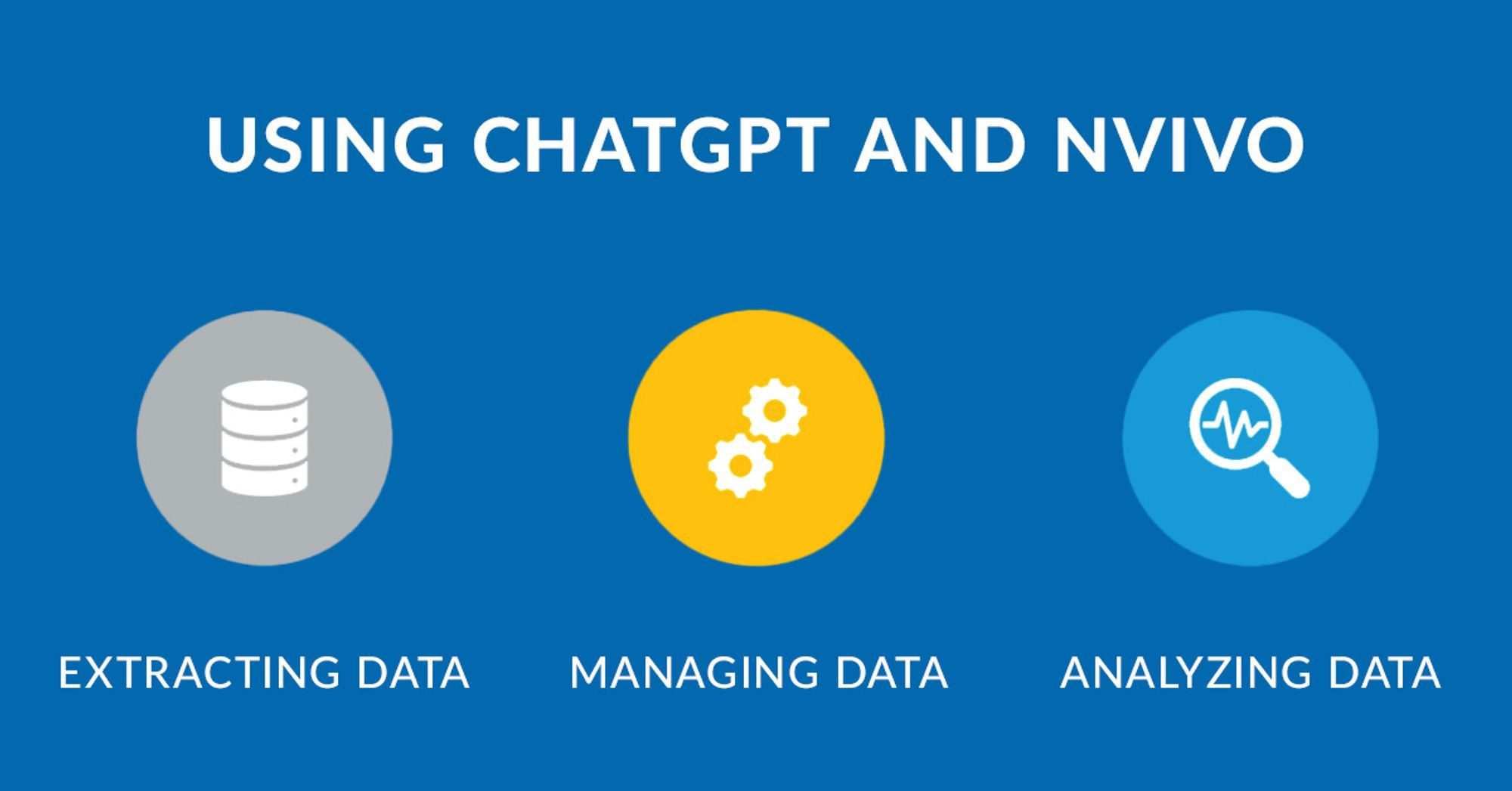
Since its introduction in November 2022, OpenAI’s ChatGPT software started revolutionizing a wide range of industries, from internet searches and customer service to software development...
ecorded interviews are one of the most popular forms of qualitative data collection. They are nearly always transcribed, and the analysis is conducted on the...

As the demand for deeper understanding and nuanced insights grows across sectors like education, business, healthcare, and government, the value of qualitative research skyrockets. Grasping...

Document analysis is the process of reviewing or evaluating documents both printed and electronic in a methodical manner. The document analysis method, like many other...

Go Forwards in Time with Citation Tracking As it’s vital for researchers to consult a variety of external sources when conducting research, such as in...

On any given day, close to 80% of NVivo users are busy with interview analysis. Like you, they're looking for the best way to make...

Learn about the stages of qualitative coding in this post with Dr. Philip Adu, Founder and Methodology Expert at the Center for Research Methods Consulting,...
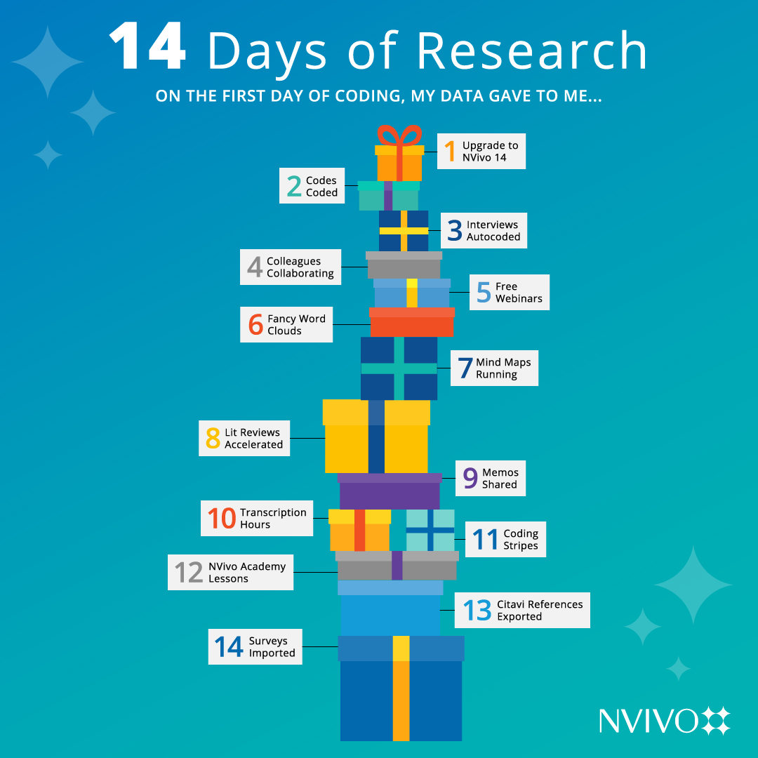
On the first day of research, my data gave to me... Join us as we help you to (re)discover some of the key elements of...

Using grounded theory, you can examine a specific process or phenomenon and develop new theories derived from the collected real-world data and their analysis. Grounded...
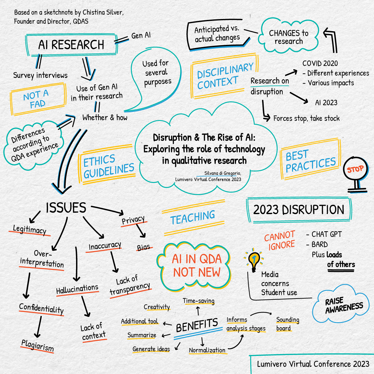
Author: Christina Silver, Ph.D., Associate Professor (Teaching) & Director of the CAQDAS Networking Project At the recent Lumivero conference, a few presentations discussed the role...

Conducting a thorough critique of the literature is incredibly important, but as a writer, you may feel daunted by the enormity of the task. Following...

Writing a literature review can be one of the most daunting aspects of the academic research process—and one of the most misunderstood. Dr. Robert Thomas,...

The practice of thematic analysis is widely used in qualitative analysis but sometimes not acknowledged or confused with other approaches. Here at Lumivero, we break...

In our fast-paced digital world, we're drowning in a sea of text data every day. Handling unstructured data manually is a daunting task – it's...
Qualitative Data Analysis Software (QDAS) allows researchers to organize, analyze and visualize their data, finding the patterns in qualitative data or unstructured data: interviews, surveys,...

Save valuable time in your data analysis with three new features and three feature improvements in part two of the latest XLSTAT release! Now you...

Anticipating Project Manager Issues with Monte Carlo Simulation to Meet Deadlines and Plan Contingencies Project management is a multifaceted endeavor that involves careful planning, resource...
Learn about Dr. Bhattacharya’s qualitative research in the field of decolonizing and gain insights into balancing research, mentoring, and supervision. In the realm of research,...
Effortlessly improve your decision making through risk modeling and analysis with @RISK software – a powerful add-in tool for Microsoft Excel. By using the Monte...

As 2023 progresses, manufacturing companies continue to focus on supply chain management issues. In an April 2023 survey conducted by CNBC, only 36% of supply...

If you’re wondering ‘what is a literature review’ or trying to figure out how to write a literature review, you’ve come to the right place....

Lumivero Support Center Now Live on the Lumivero Community Site We’re excited to announce a powerful new customer support center for NVivo, Citavi, and Sonia...

Develop your data analysis skills and connect with experts across industries at the free, Lumivero Virtual Conference! The conference spans two full days from Sept....

Deep Sensory Analysis Made Easy + Speed Up Your Sensory Data Preparation If you’re struggling with deep sensory data analysis or spending excess time adapting...

The increased costs, lack of reliable transportation, and scarcity of supplies all clearly tell the story that’s reigned on news feeds since 2020; The global...
A Conversation with Dr. Dana Lanell In a recent podcast episode, we had the privilege of delving into the complexities of the evaluation profession with...

How to Optimize Production and Inventory and Improve Tolerance Stacking Through Risk Analysis and Forecasting Supply chain management issues continue to be top of mind...

How to Keep Supply Chains Flowing Amid Global Threats with Risk Analysis for Optimizing Manufacturing For manufacturers, COVID-19 revealed many vulnerabilities in today’s complex global...

You already know that your favorite statistical analysis tool is packed with features to help derive new insights from your data, but are you using...

Free NVivo 14 Tutorials The NVivo you know and love is better, faster, and more rigorous than ever. With new team collaboration capabilities, Citavi integration,...

Organizations of all types use analytics to approach decision-making more objectively, accurately, and confidently. These techniques help decision-makers at all levels to be better-informed and...

According to Wikipedia, data analysis is “the process of inspecting, cleansing, transforming, and modeling data with the goal of discovering useful information, informing conclusions, and...

Research and technical writers at every level across all disciplines and industries experience the unique challenges of academic and professional writing – finding the right...

Behind the Data Podcast, Episode 52: TikTok Microvlogging to Engage Non-Profit Stakeholders On the most recent episode of NVivo’s Behind the Data Podcast, Dr. Stacy...

Working in a research team can be a rewarding experience, but it can also be challenging. Here are ten tips for research teams to work...
A new version of @RISK is available with advanced features for ScheduleRiskAnalysis– allowing you to apply powerful risk analysis to your project schedules.
The industry-leading risk analysis software is now even better! With more than 35 years of continuous software development, @RISK stands the test of time and...

We’re excited to announce that a new version of XLSTAT is available! Thanks to our users’ suggestions, XLSTAT is constantly improving and building upon its...

Work placements can be one of the most rewarding experiences – and most daunting – in a student’s life to date. It is likely to...

Streamlining the Dissertation Writing Process In a groundbreaking study on IT auditor competency, audit quality, and data security, Dr. Blake Curtis discovered a significant technical...

The long-term weather forecast can be summed up in one word: extreme. According to the Environmental Protection Agency (EPA), years of research into the impact...
The recent Silicon Valley Bank and Signature Bank crisis sparked significant concern and sowed distrust in the financial system among both the banks’ customers and...

In Light of the First Republic Bank, Silicon Valley Bank, and Signature Bank Crises The recent First Republic Bank, Silicon Valley Bank, and Signature Bank...

The newest version of NVivo is a significant step forward in an age when collaborative research is critical. As we bring NVivo 14 to the...
Wir haben Citavi 6.15.2 veröffentlicht und laden Sie ein, diese Version zu installieren, um die unten aufgeführten Fehler zu beheben. Falls Sie nach dem Öffnen...
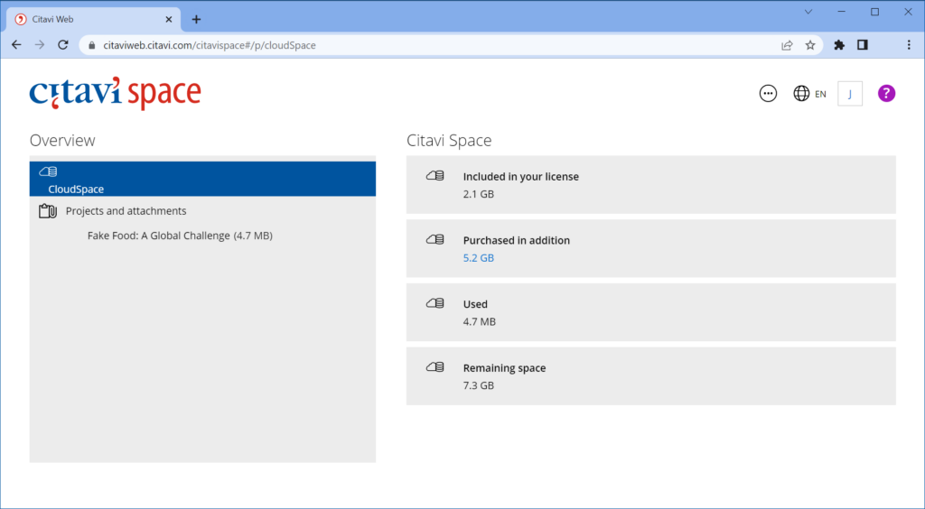
We just released an update to Citavi 6 (Citavi 6.15.2). We encourage you to install this version so you can take full advantage of the...
Managing uncertainty in project schedules has never been easier thanks to DecisionTools Suite’s newest feature, ScheduleRiskAnalysis (SRA). SRA lets you perform risk analysis using Monte...
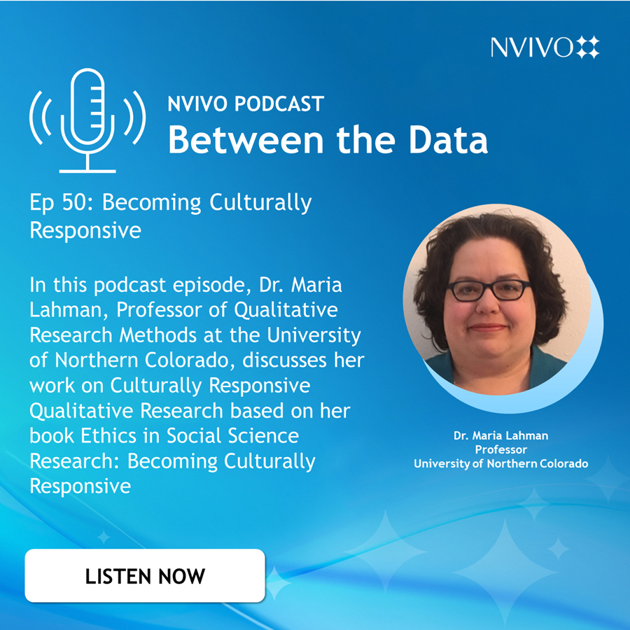
What is Culturally Responsive Research? Conducting culturally responsive research is crucial when working with vulnerable populations in order to support and respect the participants’ experiences....

Xanne Janssen has been awarded $25,000 over two years – hear from her about the study she is conducting. Xanne Janssen is a Senior...

Take charge and delegate tasks to your new personal research assistants Once you've done the bulk of your research and are heavily involved in the...

How can I find the journal article my professor mentioned? My professor recommended a journal article for my research paper... but she didn't mention the exact title, author, or journal name. Now how...

Let your sources' bibliographies do your searching for you Do you often feel like you’re searching for sources in the all the wrong places? Or maybe...

Tips for saving webpages, blogs, and articles We all know people who prefer to print things they find online before reading them. For me, it’s...

Three Solutions for Inadvertent Pilers Are your stacks of papers and books growing at such an alarming rate that you're worried about being buried alive...

And other questions regarding self-citation You’re an undergraduate student with a double major in Political Science and Chinese Studies. You write a research paper for...

Use summaries to better understand difficult academic texts On Monday morning my co-worker asked me about my weekend, as he always does. I replied, “I...

Stop pulling all-nighters for good “Guess I’ll just have to pull another all-nighter,” was a phrase I said all-too-often during my studies. It seemed that...

Two approaches for starting your writing sessions Now that it’s summer, if you’re a graduate and postgraduate student, you’re likely settling in to a writing routine to try to make progress on your dissertation. When your...

Don't buckle under the strain of your thesis or other large endeavor! Start feeling better now with our tips. After grad school I thought the...

Our 6 top tips for a successful new semester A new academic year is a great chance to start over. It’s a time to say...

All about Academic Writing Month For many academics, the month of November is associated with making progress on a writing goal. In this blog post,...

8 strategies that can help Nearly all of us have been there: sitting in front of the blank page not knowing where to start, a growing...

How to make sure you don't forget anything important Is the deadline for your research paper or thesis getting closer and closer? In an ideal...

Taking your research paper one step at a time Whenever it’s morning in the office and the telephone is ringing, countless emails remain unread in...
Why smartphones are so distracting and how you can build your concentration skills Think back to the last time you were really concentrated on your writing and completely in the...

Metacognition, metalearning, and learning how to learn Fluent in 3 months, the 4-hour chef, The first 20 hours, Ultralearning – books on rapid learning often reach the top...
How doing nothing can help you reach your academic goals. As a student, professor, or researcher it’s a given that you need to work hard....

How the fresh start effect can help with your New Year's Resolutions I am willing to bet money that no one gets into New Year’s...

11 tips to help you get the most out of your citation software Reference management programs are one of the best tools an academic can...

Three steps for taking control of a growing collection of sources. It's go time. Your advisor's parting words are still ringing in your ears, "Good luck...

The single best piece of advice for getting unstuck when writing a dissertation – or anything else A while back I wanted to start doing...

Try the Creativity Tip that Helped David Bowie get Unstuck You’ve been there before. Your sources are spread out before you, you’ve done the reading,...

Why you should avoid secondary citations Did you hear what Anna said? I heard from a friend who heard from her boyfriend’s brother that she...

How the information literacy skills you learn in your studies can help Amidst all the uncertainty of the current pandemic, one thing has become crystal...

What you need to know before using reference management software Imagine you want to hang up a picture, so you pick up a hammer to...

Whenever I start a research paper, I either feel like I can’t find anything on my topic or that I'm only finding useless information. Am...

A selection of posts from the first year of the blog The blog team is taking a break this week, but we dove into our...

Reading on screen versus on paper may impact how much you remember. Here’s what you can do. Coursework and research projects require a lot of reading. As more and more articles and books become available in electronic format, it's likely you’ll be doing much of this reading on a screen. However, research studies have shown that you may retain less information when you read something on screen rather than on paper. Reading on screen versus on paper Researchers have found problems with retention when reading onscreen materials. One study of tenth-grade students found that they had better recall and had better reading comprehension when they read a text on paper versus on screen. Another study from 2005 looked at changes in reading over the course of the last ten years. It showed that when people read on-screen, they tend to jump around more in the text rather than reading in a linear, focused manner. ...

Knowledge beyond the ivory tower Whenever I watch someone perform a magic trick, I wonder, “How did he or she do that?” In vain –...

Helpful online tools for academics When was the last time technology left you stranded? For me it was when I was stuck on hold with...

Nine questions that can help you find the perfect fit It’s not easy to find just one pair of shoes that’s right for every occasion....

Making sure everyone has a piece of the (knowledge) pie Imagine that you buy a bushel of apples from your local supermarket and then bake...

When to use them and what to watch out for Whenever I hear the term “social media” I think about the platform I personally use...

And how your reference management software can help In our last post, we looked at some strategies for being more creative from the book Creativity in Research....

And how you can find peer-reviewed journals for your first research paper Did you just get assigned your first research paper and are wondering about...

Start off your studies strong Being a first-year student is difficult enough when you don’t have a pandemic going on around you. You have to...

What to focus on for long-term change, plus helpful tips you can use now Academic research requires creativity. Whether it’s putting together an original research...
Schnell und langfristig kreativer mit diesen Tipps Ohne Kreativität gäbe es keine Forschung. Wenn Sie Ihre Forschungsfrage formulieren, einen neuen methodischen Ansatz austesten oder eine...

Reach great heights by building upon the achievements of others As a student, you may often feel daunted by your professors. During my college years,...

A look at the Planned Accidents blog authors' idea generation and writing process In this third post in our creativity series, blog authors Jenny and...

5 tips for Citavi (and other) webinars This blog post is especially meant for Citavi instructors, their colleagues, and future Citavi Champions who want to share their...

Who gets thanked in the acknowledgements section in theses and dissertations and why As a Citavi customer proudly told me that he had completed his...
Since the beginning of the year there have been a lot of changes made to Citavi, which we're excited to tell you about in this...
Dissertation writing requires you to develop a complex argument supported by appropriate evidence. To do this effectively, you’ll need to learn how to organize your...
Most of us can imagine the academic who effortlessly turns caffeine into written words and might actually be a machine. It’s easy to think that everyone else...

Updated: Sept. 1, 2023 The escalation of Russian’s invasion of Ukraine and the ongoing response to the COVID-19 pandemic contributed to crude oil price volatility...

Evaluation of Student Success within Social Work Education’s Signature Pedagogy Over 250 Sonia users came together in October to share best practices and learn more...

Evaluation of Student Success within Social Work Education’s Signature Pedagogy Field education is the “signature pedagogy” of social work education (CSWE, 2008). As a result...
Between the Data Episode 47: Post-Intentional Phenomenology: Considerations and Principles Social science researchers have long utilized phenomenological research methodologies in their qualitative research to study...

Continuing with this series of articles introducing cost estimating with @RISK, we will compare the use of the most popular distributions of this technique: the...

Academic Writing Month runs in November and challenges participants to set and meet a writing goal during the month. To help everyone participating, we’ve done...
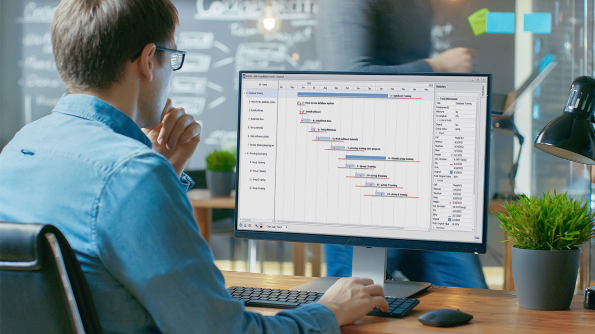
Manage uncertainty in project schedules like never before with Monte Carlo simulation. Perform risk analysis on Primavera P6 or Microsoft Project models in the @RISK...

Beauty has long been a topic of interest, from philosophers who struggled to define it to artists who sought to portray it. And now, with...

Originally Published: Nov. 1, 2022 Updated: Sept. 1, 2023 At the time of this article's publication in November 2022, the U.S. dollar was at its...

This article offers a simple and concise explanation of the Monte Carlo simulation, a technique that combines statistical concepts (random sampling) with the ability of...

The 2022 FIFA World Cup is right around the corner and the tournament predictions are pouring in. While checking team rankings and relying on gut...

NVivo was used to enable a recent study that identified family history as the most significant factor in assessing personal breast cancer risk, but health...

The fear of the blank page, the stress of self-imposed writing goals, perfectionism - all of these can prevent academics from engaging in productive writing...

As the world of work moves ever faster, it’s never been more important for academia to connect with business and the workplaces into which students...

A Purchasing Strategy Example Considering Suboptimal Decisions Lumivero’s PrecisionTree software allows you to analyze the probabilities of different outcomes, and their impacts, in sequential, multi-stage...
Dr. Janet Salmons interviewed by Dr. Stacy Penna, Engagement and Enablement Director NVivo Podcast Between the Data Ep 44 Launched by SAGE Publishing in 2009,...
Real estate investment opportunities come in all shapes and sizes – from new developments that traditionally provide reliable, predictable income, to troubled properties that could...
Dr. Pablo Valdivia & Rosmery-Ann Boegeholz interviewed by Dr. Stacy Penna, Engagement and Enablement Director NVivo Podcast Between the Data Ep 43 It’s hard to...

Scholarly Writing Institute Recap Enhance your writing skills and discover digital tools to assist with the publishing process. NVivo and Citavi have once again partnered...

Many who have been exposed to Monte Carlo simulation learned about it in the context of financial modeling such as asset management, cash flow analysis,...
A common first step in litigation strategy is to calculate the case’s settlement value. As discussed in our past legal blog series, settlement calculations can...
Previously we discussed the importance of crafting decision trees in litigation strategy and why patent litigation is an expensive, time-consuming process. In part three, we...

To lay the groundwork for swift settlements, many legal firms use PrecisionTree software to map out all possible routes a litigation path can take by...
In litigation, you often get stuck in inefficient negotiations. Between 95-97% of patent lawsuits settle before trial, but not before amassing an average of more...
Business continuity and emergency response managers know that recovering from a crisis requires proactive planning – regardless of whether you can see trouble approaching. Lessons...

Enhance Your Research Grant Funding Application with Lumivero Across all disciplines, there is growing pressure to obtain grants to advance research. There are many reasons...

I have been helping academics and others on their writing and writing productivity for over twenty years (and over ten years as a coach--time flies!!)....

Long supply chains for technology companies in the United States combined with the need for timely delivery of products to customers has brought challenges to...

Setting aside the issue of expertise, even mid-career academics have a hard time imagining how they could make the investment of time to write a...

November is Academic Writing Month (AcWriMo)! Along with the bounty of resources and advice that Academic Writing Month brings, it is important to acknowledge the...

After joining the newly formed Boston University Wheelock College of Education and Human Development, I was tasked with leading a project to centralize and streamline...

We’re delighted to have our new Product and Community Director, and field placement expert, Sally Warlow, presenting a webinar on how she spearheaded an initiative to...

This is a continuation of Part I in this series on Decision Tree Analysis. Life is full of tough choices. Most of us muddle through...
Conducting analysis of decision making under uncertainty using decision trees serves several purposes. This can be done easily in Excel spreadsheets with PrecisionTree software. First,...
The use of custom Excel programming and @RISK APIs allows the automated analysis of historical data and construction of sophisticated risk models. Here, we present an application...

Create a Better Field Placement Experience Improving field placement communications with the right plan, framework, and approach can help save time, increase productivity, and create...

Field placements, experiential learning, student placement or work-integrated learning – it doesn’t matter what you call it, on-the-job learning for students is fast expanding and...

Palisade's former CEO, Randy Heffernan, was featured in the May 2021 issue of Risk Management Magazine. In this article he shared, in part: Monte Carlo...
Utilizing a software called @RISK we evaluated the NASA bearing data to determine the best-fit distribution. It turns out that for the bearing data, the...

The prospect of graduating from spreadsheets or sticky notes to placement software is exciting. There are so many time and cost savings, plus the ease...

With Citavi now part of the QSR International family, we’ve released a new NVivo and Citavi integration into the latest version of NVivo (released in...

I don’t know a researcher on the planet who doesn’t wish they could publish faster. If you work with NVivo, you already know that it...

We are very pleased to share exciting news: QSR International has acquired Citavi, the only all-in-one reference management and note taking app that will intuitively...

Back in 2000, I wrote about how you could you use NVivo for your literature review. The software has changed significantly since then with a...

When it makes sense to cite manually or use an alternative Our team regularly monitors Twitter for discussions about the use of reference management software...

Asking the right questions is the first step Early on in your academic training, you may have been assigned topics to research. As you progress...

Our recommendations for working with URLs Gone are the days of citing only printed materials when writing a research paper or thesis. Depending on your...
Palisade’s PrecisionTree is used help decision makers choose between multiple options and take account of cost and rewards of different options, such as choosing the highest...

Confronting the myth of the lone researcher There is a myth that qualitative researchers work alone. Lyn Richards, co-developer of NUD*IST and the early versions...
When our Field Education team had the opportunity to improve inefficient processes that were adding time and costs to running our field placement programs, we...
When our Field Education team had the opportunity to improve inefficient processes that were adding time and costs to running our field placement programs, we...

It’s that time. Accreditation season. You’re preparing. Where are those assessments stored? How do you find that data? The pressure is on to ensure your...

People managing placements are busy! There are students to manage, site contacts to update, sites to source and university staff to report to. Often, entire...
Calum Turvey, W.I. Myers Professor of Agricultural Finance, uses @RISK in his Risk Simulation and Optimization course. Offered by the Charles H. Dyson School of Applied Economics and...

It’s never been more necessary to ensure strong risk management in a placement program. Universities and workplaces are managing numerous unknowns, and operational requirements can...

Why Centralized Placement Management Is the Future Higher education institutions are prioritizing student experience, teaching innovation, diversity and workplace readiness. Key programs of work to...

7 methods for taking notes in class Do you dream of doing better on tests and getting better grades? According to a recent study by...
The basis of a solid risk assessment is understanding that probability exists in a range, not a specific number, says Henry Yennie, a program manager...

Experiential education programs are vital for effectively preparing students for the workforce. Managing these programs can be challenging, and how students and host sites experience...
Hospital bed availability changes daily, especially during COVID-19, as patients are admitted and discharged. @RISK gives staff a real-time look at data as it evolves,...

What beginner’s mind is and how can you apply it to your long-term projects A couple years ago I did something way outside of my...

To support researchers all over the world in coming together, we are hosting our first virtual conference, “Qualitative Research in a Changing World” on September 23,...

The blueprint for your writing project In everyday language, the word “proposal” is probably most frequently used in the context of marriage or business. In...

Our tips and favorite tools for task lists Is there any better feeling than finally finishing a task you had been putting off for a...
This is an example of the use of @RISK automation applied to stock portfolio optimization. It is a custom application written by Lumivero Custom Development...

There are tens of thousands of citation styles. Why are people still developing their own? Whenever I teach a course on Citavi, I ask the...

In the Empowerment Through Culturally Responsive Focus Groups podcast, Dr. Jori Hall, Associate Professor at the University of Georgia in the Department of Lifelong Education...

Form your own academic dream team Who doesn’t love a good heist flick? A team of misfits, each with their own unique specializations, gets together...
Methods for annotating academic texts Do you have any academic guilty pleasures? During my studies, I certainly did: highlighters. I absolutely loved marking up my...

QSR has long been committed to making NVivo intuitive and easy to learn. The newest version of NVivo, released March 2020, includes five sample projects which illustrate how NVivo can be...

A Change Of Scenery Changing your workspace can have wide-ranging benefits—from enhanced mental and social stimulation to improved productivity, focus, and creativity. Gone are the...

Easily find all of your handouts and other class materials with your reference management software Under normal circumstances, how do you typically deal with all...

In the webinar focused on the impact that the COVID-19 crisis has on researchers, Christine Hine, Professor of Sociology at the University of Surrey, UK,...

Why we avoid it, why we shouldn’t, and strategies to get through it At the time of writing, Switzerland continues to recommend staying and working...

During our webinar titled Teaching Qualitative Methods Online a panel of instructors discussed best practices on incorporating QDA software, like NVivo into an online qualitative methods...

We interviewed Jim Cockell, who is part of a research team in the Faculty of Nursing at the University Alberta. The research team works with...

During our recent webinar on COVID-19 and Virtual Qualitative Fieldwork, Dr. Deborah Lupton, Professor at the Centre for Social Research in Health and Social Policy Research...

In the second webinar of our series focused on the impact that the COVID-19 crisis has on researchers, When the Field is Online, Dr. Janet...
Modeling from empirical data takes observed information and attempts to replicate that information in a set of calculations. There are a number of relationships to...

Kristi Jackson, trusted NVivo expert and trainer has reviewed the new NVivo and shares her thoughts. A Visual Delight Import > Organize > Explore! This...
Get the most out of the e-learning experience When we published our last blog post two weeks ago, the world was a very different place...
Each March, office productivity is greatly impacted by the NCAA Men’s Basketball Tournament. Just about everyone—regardless of their passion for college basketball—fills out a bracket in...

A look at why attempts so far have failed If you travel to Germany and order a beer, you might notice that the glass has...

Why it can be problematic and when it can make sense When you’re first learning how to write academic papers, you’ll often be told to...
An achievable resolution for the new year At the beginning of a new year, there’s often the temptation to formulate resolutions: do more exercise, stop...
The continuous uniform distribution represents a situation where all outcomes in a range between a minimum and maximum value are equally likely. From a theoretical...

Give the students, professors, or researchers in your life a present they’ll love! If you’re an academic, chances are that you also know an academic...
A brief history, from the very first guidelines on up to APA 7 The APA citation style just might be the most widely-used citation style...
In Six Sigma analyses, there seems to be some low level confusion about Cpk and Ppk and what they actually represent. Very basically, Cpk is...

Think outside the box and develop your own system of keywords or labels We like to put documents – and people – in boxes. This...
Navigating your way through the long, difficult parts of a semester When I was a student, I remember being full of motivation at the start...

When performing a cost risk analysis study, one of the key results is the amount of extra monetary resources that is to be added to...

Tables of contents, lists of figures, and other "signposts" for your text If you’re in a new place, you’ll often spend a few minutes trying...

An itinerary for your writing journey Whenever I have a vacation coming up, I create a rough itinerary for myself. I decide where I want...
Real options are the flexibilities that are inherent in general business or other decision situations. In general, a real option is present in any decision...
What are the characteristics of successful managers? Surveys consistently show decision-making ability at or near the top of the lists. Perhaps no management activity is...
When building a Monte Carlo simulation model in @RISK for project risk analysis, we can incorporate a risk register through risk factors. Risk factors are more concrete...

…and add difficult sources to your referencing software like a pro Librarians have a gift. They can take one look at a source and know...

Citation terms explained in plain English As a university student, you’re expected to adhere to citation style guidelines for your papers – but that can...

...and how it relates to reference management During an internship at my university library, I used to lead training courses on a particular reference management...
Let’s move on from Part I of this blog series on the Efficient Frontier, formulated over half a century ago by Harry Markowitz, to the...
This article from IndexUniverse.com details just one of the ways Monte Carlo simulation can be tuned to the combined unfolding of time and risk. First, a little...

When publishing your work is a bad idea “We would be delighted to publish your thesis as an academic book.” One of my peers read...
In Part II of this series, we mentioned the existence of an analytic method to calculate the Efficient Frontier of a portfolio. Here we provide...

This entry follows on from Part I, describing portfolio optimization for portfolios where the expected return and standard deviation are sufficient to describe the decision-makers’...

Organize your reference database with our 10-step checklist If your reference management program were a closet, would it look like this? Or more like this? If it's...
The topic of the selection and weighting of assets (or projects) associated with an optimal portfolio is a large and complex one. For example in general business...

Dr. Philip Adu is a Methodology Expert at The Chicago School of Professional Psychology (TCSPP). In this post he explains the things to consider when...
This blog briefly posts some fairly standard “best practice principles” in Excel modeling. The following principles are generally to be applied to Excel models (in...
Just for fun, here we talk about using Monte Carlo simulation to estimate the value of π (3.14159…). A circle of radius one will have...

What place does Wikipedia have in academic writing? When you start a research paper, you may not be very familiar with your topic. You’ll want...

Celebrate your best moments and thwart the negativity bias As we stand on the threshold of a new year, many of us have already thought...

Get your sources under control in 2019 Did you make resolutions last year that you never saw through? Everything will be different this year! We’ve...

Tips for recognizing, adding, and citing different reference types The sources you use to write your paper are a bit like road signs. Just as...

NVivo Transcription has arrived to help solve the problem faced by many researchers – hours of manual transcription of data sources like interviews, and focus...

Proofreading and copyediting can make your work really shine. Here's what you need to know. There's nothing like typing the last sentence of your thesis...

Three methods and when to use each one Did you know that the British Library is the largest library in the world with over 150...

Writing a Thesis with a Company Citavi Support team member Jana works every day to make your academic research easier. Her journey to Swiss Academic...

10 Tips For Staying Productive on the Go Summer, sunshine, vacation... as soon as you finish up that one thesis chapter, that is. If time...

Best practices for collaborating with colleagues, data source considerations, and sharing actionable insights for healthcare and non-profit researchers Collaboration and stakeholder management Engaging in a...
Renewables pose real challenges for utility operators, particularly solar and wind power. Renewables such as biomass, geothermal, and hydro, however, are as controllable as fossil...

NVivo and SPSS both feature heavily in the toolkit I use as a researcher, so I was pretty excited when I heard that NVivo would...

Just pick a citation style and let your computer take care of the rest! It’s 12 a.m. You’ve got a paper deadline, and, luckily, all...

Top Tips for Successful Teamwork People rarely feel neutral about meetings, collaborative projects, and shared presentations. Many have a love/hate relationship with teamwork. The pros...

Keep track of what you read and prevent plagiarism You’ve got a pretty good memory, don’t you? You know exactly what you ate for breakfast...

The new NVivo 12 is here, and I’m very excited to share with you all the new features and improvements that are available across both...

Setting Up a Paper-Writing Workflow Large writing projects can seem overwhelming. There’s so much to do that it can be hard to know where to begin. One...

Accidents are part of the research process. Many breakthroughs come about unexpectedly or by mistake. Wouldn't it be great if you could more consistently obtain such eureka moments in your...

"None of us is as smart as all of us." -- Ken Blanchard Collaboration in NVivo 11 Pro for Windows revolves around the idea of...

University of Hull Library Skills Adviser, Lee Fallin, share his insights on creating an NVivo community via a user group on campus. The University of...

Cases and their attributes are powerful features in NVivo. They facilitate comparisons between your research participants (or other entities) and can reveal patterns and insight...

As a qualitative researcher, you wear many hats. For any given project, you need to: Read widely and have a thorough grasp on what’s happening...

Lyn Lavery is an NVivo Certified Platinum Trainer and, as the director of Academic Consulting, has overseen an extensive range of academic and government-based research...

In this blog, we take you through the ins and outs of literature reviews, what critically examining the literature means and how to get started. ...

Whether you’re a student or an experienced practitioner, it’s not unusual to have a crisis of confidence during a qualitative research project. This credibility checklist...

Dr. Sachin Kumar Mangla of the UK’s Plymouth Business School uses @RISK in his research on risk management in sustainable supply chains in India. Dr....
Coding in NVivo for Mac? Here are 6 videos to help you. 1. Find out why nodes and cases are so important Not sure what...
It’s often difficult to determine which factors require the most attention in business decisions which can lead to focusing on the wrong things while ignoring...
Project Manager Today took an in-depth look at @RISK Professional, saying: "All projects involve risks, but it’s vital to understand what those risks are and how...
Agriculture is traditionally one of the highest risk economic activities. In California, many produce farm operations use a rule-of-thumb to manage their seasonal finances–often aiming...

Yes, the new NVivo suite is here and you can choose an edition of the software that suits the way you want to work. Question...

Humans are inherently complex. Research with human subjects requires patience, attention to detail, and a love of intersectionality. NVivo helps one harness their inner zen,...
Climate change has already started to create extreme and unpredictable weather events around the globe. In this article, Randy Heffernan outlines the importance of considering...

This post started life on the NSMNSS blog—a great initiative (run jointly by NatCen Social Research and SAGE) that fosters lively discussion about the challenges...

There are some excellent resources available about using NVivo for your literature reviews. Here, I describe some ways in which I use NVivo for literature...
A large part of the risk management process involves looking into the future, trying to understand what might happen and whether it matters to an...
Analytics India Magazine featured Palisade's World Cup 2014 simulation model in their article, "How to Win the World Cup Office Pool". Taking data from the...
The world of financial markets and investments is rife with risk and reward. This is particularly true for hedge funds, sophisticated investment vehicles that are...
Soccer fans around the world are gearing up for the 2014 World Cup in Brazil. Many will be putting money on the various matches—basing their...

The Wall Street Journal featured @RISK's 2014 World Cup simulation model in their article, "The Journal's Prediction". Reporter Matthew Futterman consulted Fernando Hernández on his...

NVivo allows you to create diagrams from your data - a picture emerges of different categories and nodes and how they relate to each other....
The article shines light on the fact that the U.S. Food and Drug Administration has launched an interactive web-based tool called iRISK, to combat the...
A recent article written Randy Heffernan explores a variety of applications of Monte Carlo simulation in the manufacturing sector, such as: minimizing pilot programs, enterprise...
The Super Bowl brings a significant amount of speculation on a multitude of outcomes—from who will win the match, to what color Gatorade will be...
As green options move toward becoming the norm, new risks can result, such as whether environmentally-friendly materials can withstand a major earthquake, hurricane or flood....
Monte Carlo simulations, named for the city in Monaco, were developed during the 1940s with the Manhattan Project. But today’s simulation software can be used...

In this post, Dr Jenine Beekhuyzen explains the importance of a codebook when working in a research team. I originally began writing this blog post...
Business innovation is the lifeblood of most enterprises – and given the inherent high uncertainty, a high level of decision quality is essential. Many parties...
In light of evolving demands from customers, makers of enterprise risk management software programs are reworking their offerings with an emphasis on increased speed and...
How do businesses eliminate risk? The simple answer is this: They can't. It is impossible. Understand the nature of risk factors, and plan strategies accordingly....
Alternative Energy eMagazine interviewed Randy Heffernan about risk analysis in the energy industry. The article highlights FutureMetrics’ use of @RISK to hedge wood prices in...
The expansion of global supply chains has meant an exponential growth of the risk of disruptions to those networks. Organizations around the world are turning...
Increased use of risk analysis in the form of quantitative risk management (QRM) and decision-making under uncertainty (DMUU) is helping organizations to be prepared for...
Community services provider Arc of Yates utilizes simulation program to predict potential budget shortfalls
A South African infrastructure development company has used @RISK risk analysis software to ensure it attracts funding for projects to deliver basic community services that...
The pros and cons of energy systems have never been as critical as they are today. Energy sources, irrespective of how “green” they may or...
Risk is not an exact science, but there are specific trends that should impact decision makers.
In the world of reinsurance, accurately determining risk is critical. The application of Monte Carlo simulation is being considered more often in order to better...
This article discusses how organizations should take a more strategic approach to weather risk. Heffernan explains how Monte Carlo simulation can be used to help...
This case study takes a biofuel plant as an example where @RISK models the project's Net Present Value (NPV), PrecisionTree informs strategic scenario decision-making, and...
Craig Ferri provides a list of guidelines for implementing Quantitative Risk Management (QRM) and Decision Making under Uncertainty (DMU).
In this byline, Randy Heffernan outlines risk management best practices to ensure the success of software projects and shares tips for crafting effective risk management...
In this article, Randy Heffernan is quoted on the emerging risk management software market. The article discusses the appeal of risk management software to large...
The reinsurance industry has endured numerous larger than expected losses in the last decade or so -- everything from Hurricane Katrina to the global financial...
Given the state of the current global economy, there's been a lot of talk about the need for "proper risk analysis." The concept of risk...
@RISK is available with companion product PrecisionTree in the DecisionToolsSuite. PrecisionTree creates decision trees in Excel to allow you to map and understand the complex decision...
This article explains how 'Black Swan' events are changing perceptions of risk analysis.
@RISK’s use of Monte Carlo simulation allows for powerful features, like RiskSimtable. The RiskSimtable feature can be used to run multiple simulations to test the sensitivity...
This article explains why now is the perfect opportunity for risk managers to play a more important role in companies than ever before. Click here...

Example Model of Sensitivity Simulation: SENSIM.XLS Sensitivity analysis in @RISK (risk analysis software using Monte Carlo simulation) lets you see the impact of uncertain risk analysis model...
By now we’ve become accustomed to the marvels of neural network technology and, in fact, inured to the advances it brought in statistical analysis with...
A team of MIT scientists calling themselves Liquid Stone made a breakthrough (as it were) discovery about cement. The Romans used cement to build their remarkable...
The authors examine decision analysis methods that merely make people feel better about their decisions with those that produce measurable improvements over time. They find...
When modeling risk events, it is common that several events could affect the same cost element of a project. During the simulation, two or more...
An earlier blog on Best Practice Principles in .Excel Modelling generated quite some interest, as well as demand for more details on some of the points...
The blog positing on best practices in Excel modelling could be thought of as providing a reasonable and robust set of principles for building static Excel...
This blog briefly posts some fairly standard (but not fully accepted, and more often simply not implemented!) “best practice principles” in Excel modelling. A later...

In Part I, combining simulation and decision tree analysis techniques was introduced. But what does that actually give you? What meaningful results are created to...
First of all, what is Monte Carlo simulation? Monte Carlo simulation is a computerized mathematical technique that allows people to account for variability in their...
When using @RISK (risk analysis software for conducting Monte Carlo simulations in Microsoft Excel), one of the output graphs is a tornado graph. Such graphs...
@RISK is used to assess the relative benefits of different drilling strategies for Lundin, a small exploration company, for field development. Click here to read...
A discussion of how modelling software is having an impact on monitoring the spread of global diseases. An example using @RISK to combat avian flu...
Researchers at the University of the Pacific’s Thomas J. Long School of Pharmacy and Health Sciences used Palisade’s NeuralTools to assist in the evaluation of...
According to a recent Harvard Business School study, higher IT capability directly correlates with superior revenue growth. Nearly all IT managers (at more than 150...
This is the first in a series of articles that will examine some of the most commonly used decision-making methods for the selection or rejection...
Palisade's Mirek Janusz provides a summary of the methodology and applications of neural networks software, including Palisade's NeuralTools.
I was looking for a software tool that was easy to use and would do forecasting based on complex parameters,’ said independent health care consultant...
In this article, @RISK is used to illustrate how to plan for retirement more accurately using Monte Carlo simulation. Click here to read the article....